ECE 449/549: 2^nd Midterm: Solution - Fall 1998

1. Given the following two-port circuit segment:

   

   1. Find a bond graph representation of this circuit segment.

   2. Assuming that the currents i₁ and i₂ are computed by the environment in which this circuit segment is embedded, assign causality strokes to the bond graph. Determine whether the circuit contains:
      • algebraic loops
      • structural singularities

      We can draw the bond graph at once. The assumed causality fixes the strokes at the 0-junctions at the left and right end. The remaining causalities follow.

      

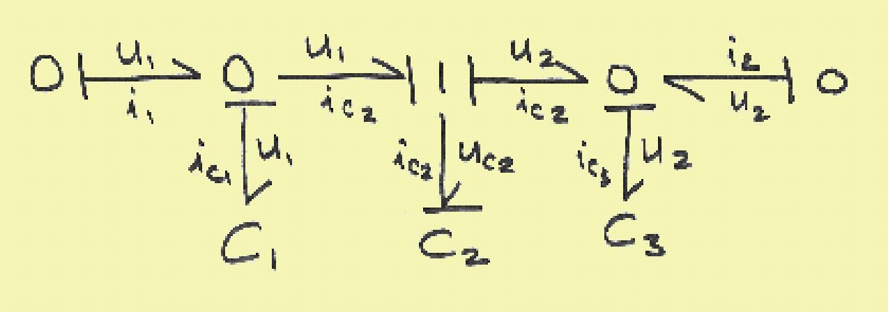
      There is an incorrect causality at the capacitor C₂. Hence the circuit is structurally singular.

   3. Show that this circuit segment can be used to realize the capacitive field:

      

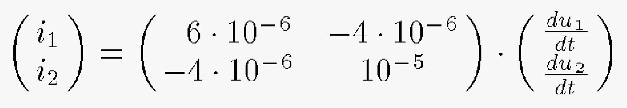
      How do you need to choose the three capacitors, C₁, C₂, and C₃?

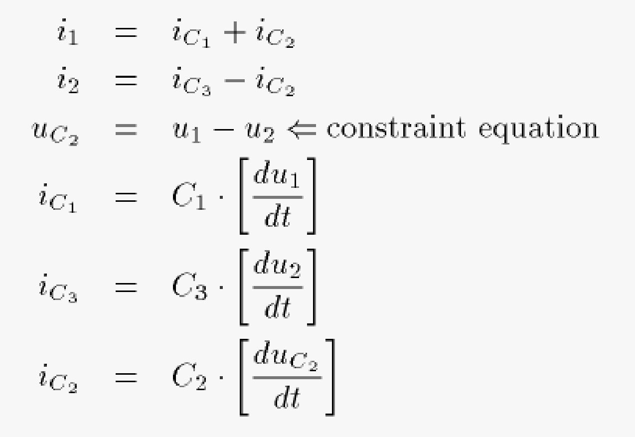
      We extract the equations from either the bond graph or the circuit:

      

      We assign as many causalities as we can. We find at once a constraint equation:

      

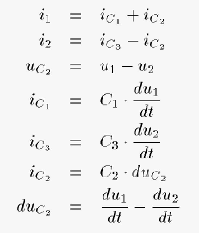
      We differentiate the constraint equation, add it to the set of equations, and relax one of the integrators instead:

      

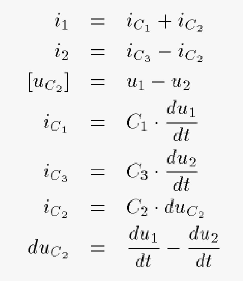
      We again assign as many causalities as we can:

      

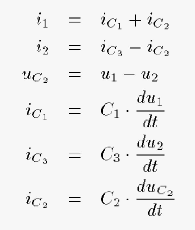
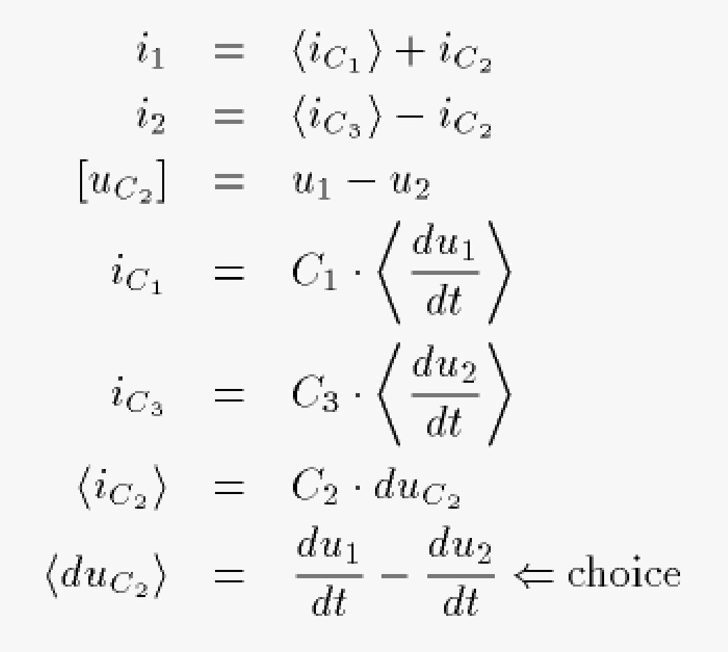
      We now end up with an algebraic loop containing 6 equations in 6 unknowns. We make a choice, and find:

      

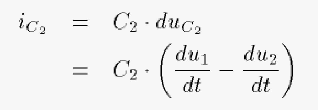
      We can solve for i_C2:

      

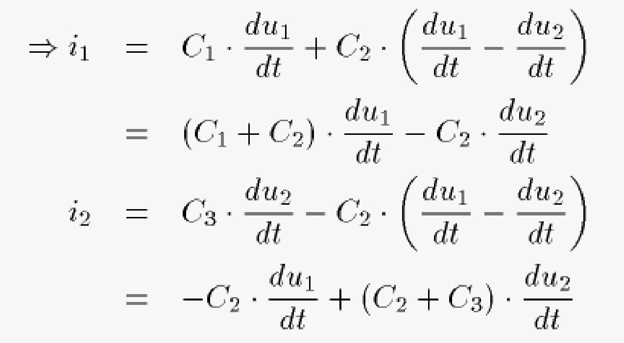
      Now, we can solve for i₁ and i₂:

      

      In matrix form:

      

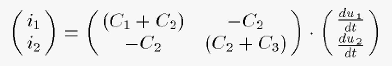
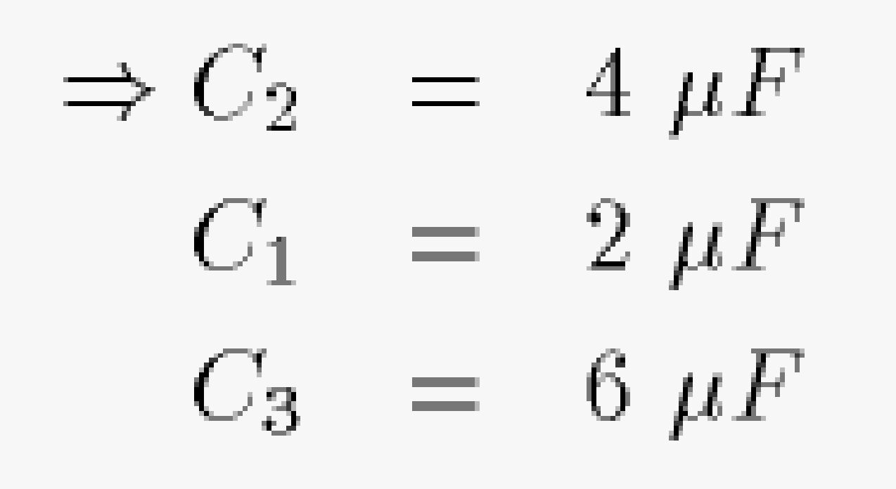
      Hence:

      

    

2. Let us start with the bond graph of Fig.7.19 in the book:

   

   For programming this bond graph in Dymola, it would be easier to work with the dual bond graph.

   1. Draw the dual bond graph with causality strokes and variables shown on all bonds.

      

   2. Augment the dual bond graph by additional 0-junctions as needed for Dymola.

      

    

3. Given the mechanical system as shown below:

   

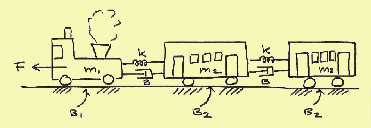
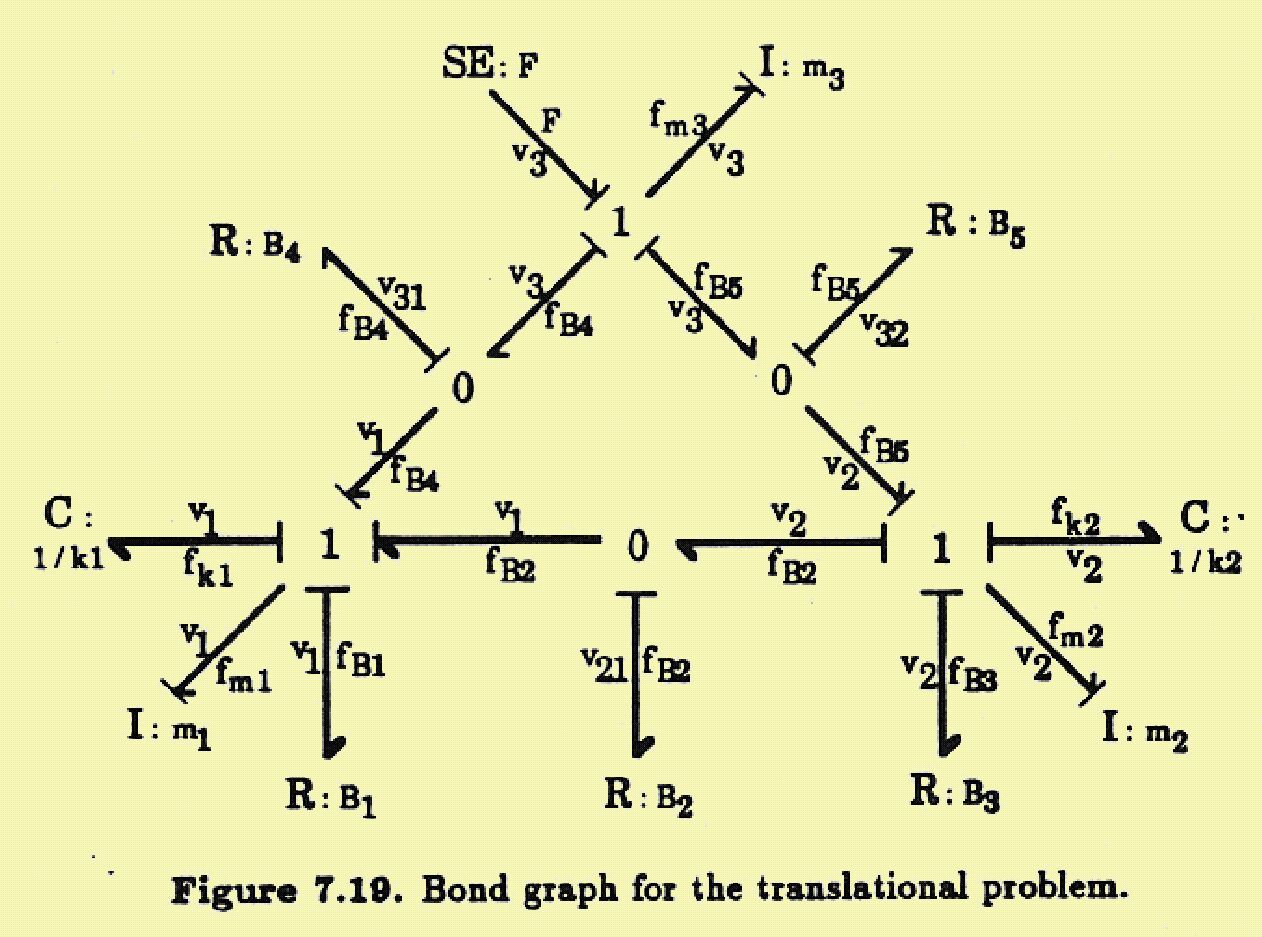
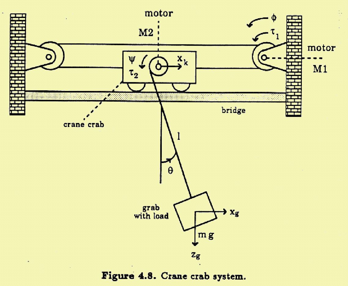
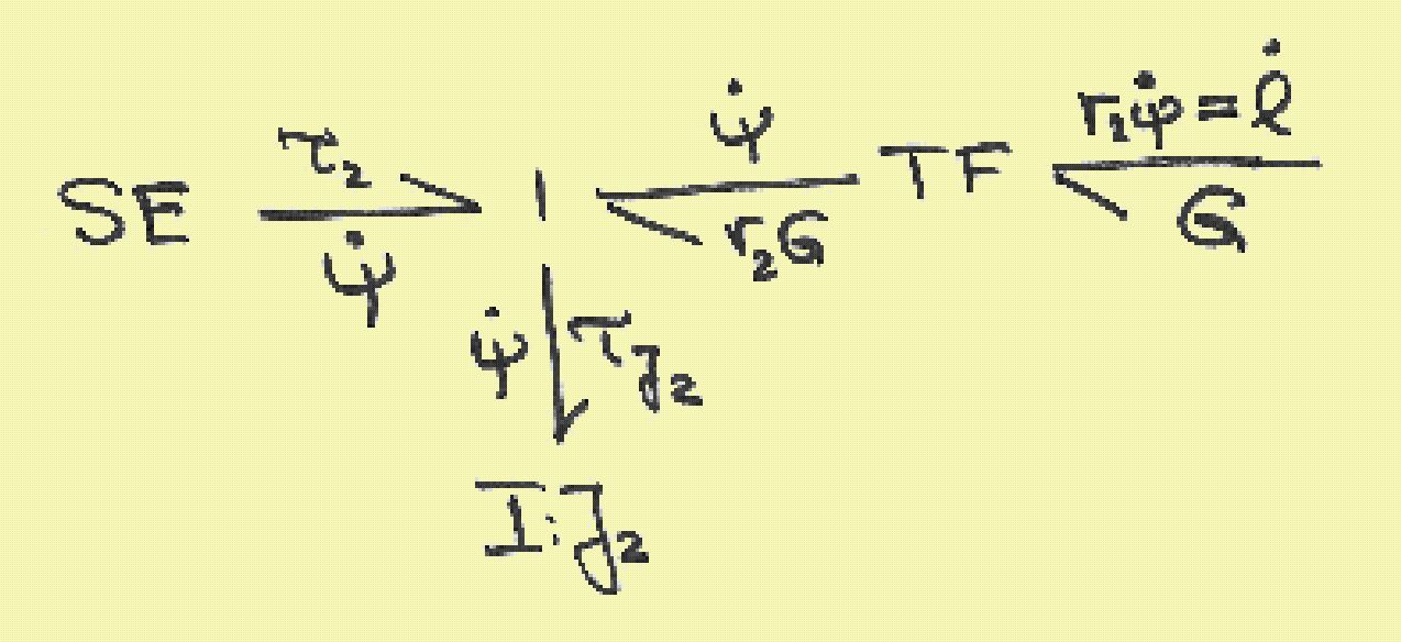
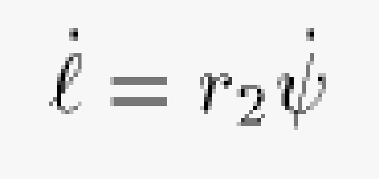
   The train is pulling two wagons behind the engine. There exists friction (a damper) and elasticity (a spring) between neighboring wagons. Also, there exists friction to the ground. For simplicity, you may ignore the rotation of the wheels.

   1. Find a bond graph description of this system.

      We start out by extracting the essential properties of this system:

      

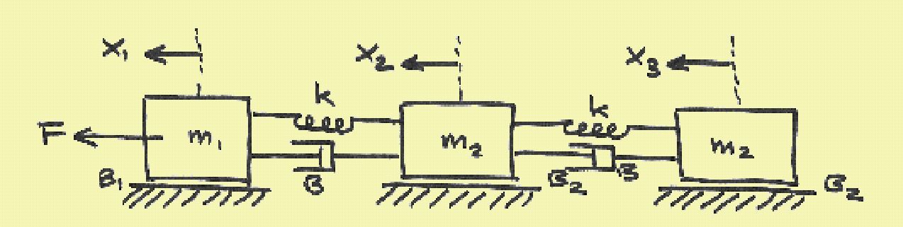
      We can now draw the bond graph directly:

      

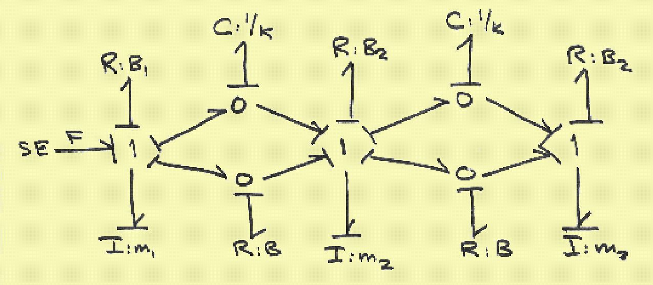
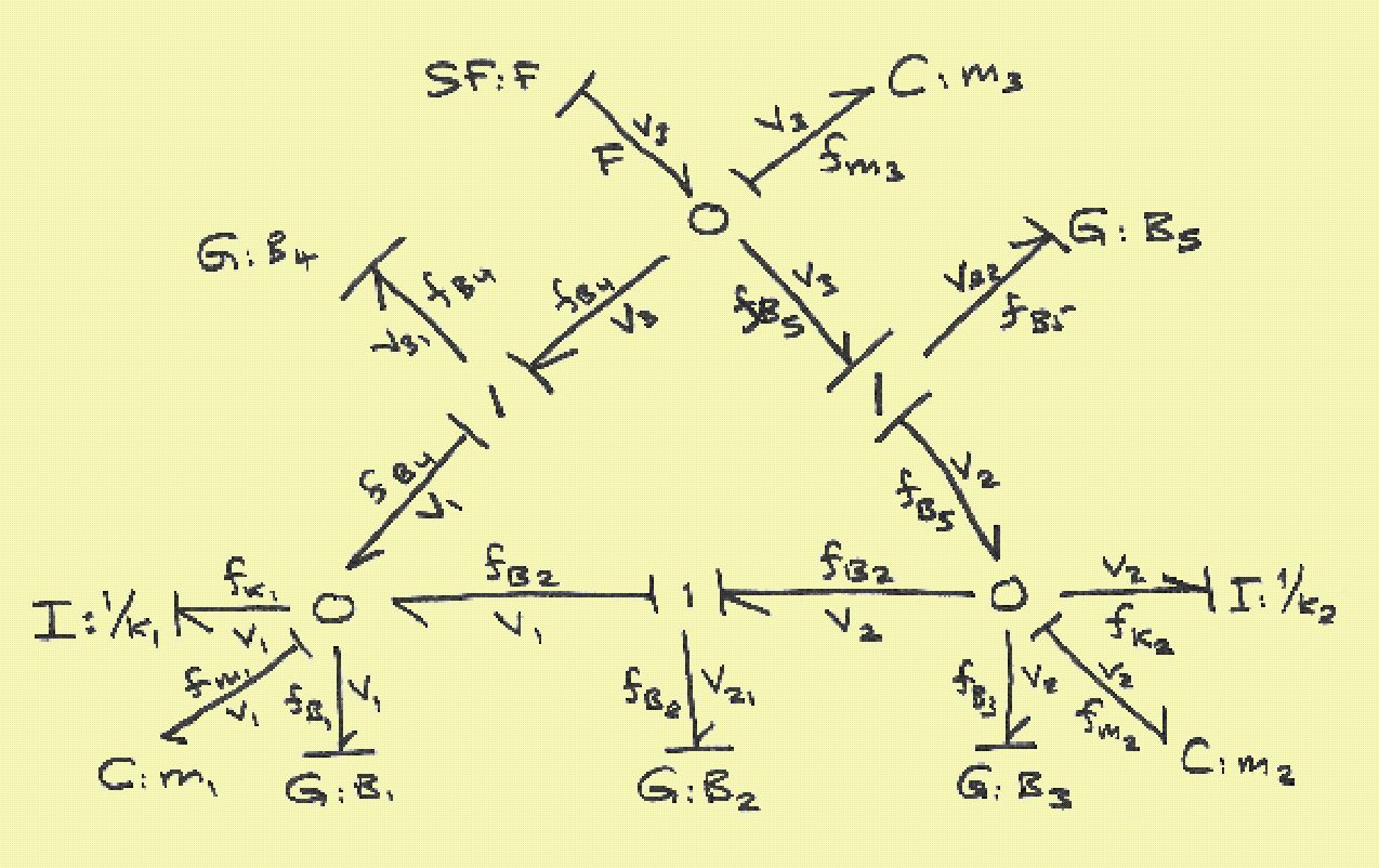
   2. Use the diamond property to simplify the bond graph found above.

   3. Add causality strokes to and assign variable names with all the bonds.

      We obtain the modified bond graph:

      

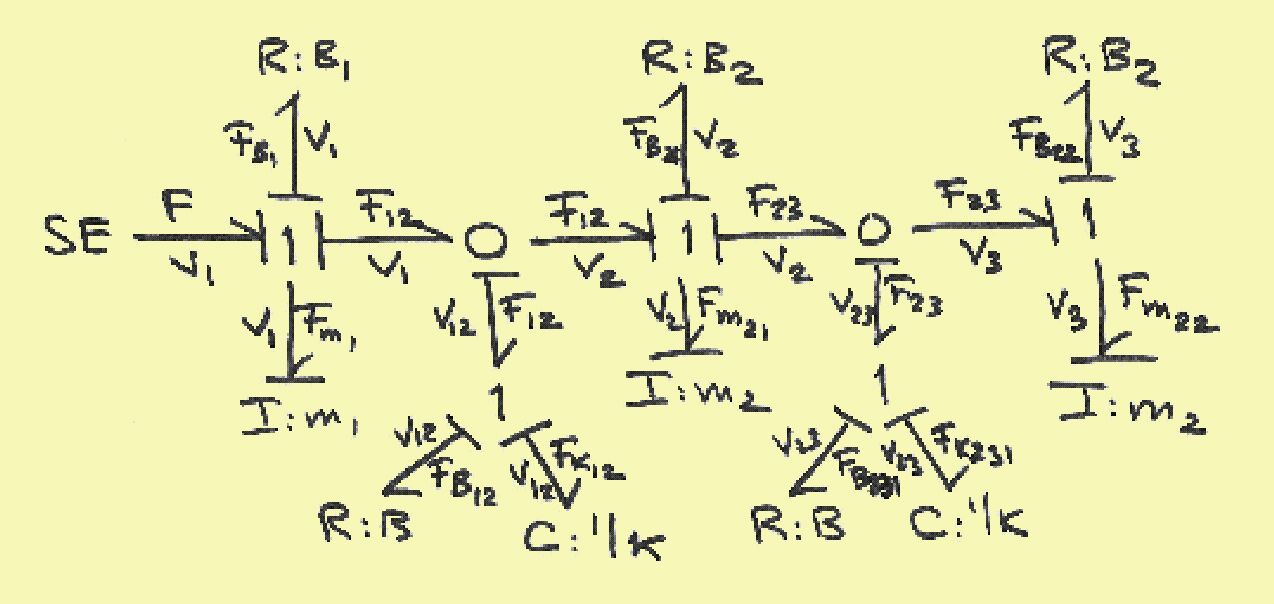
      I added causality strokes and variable names as needed.

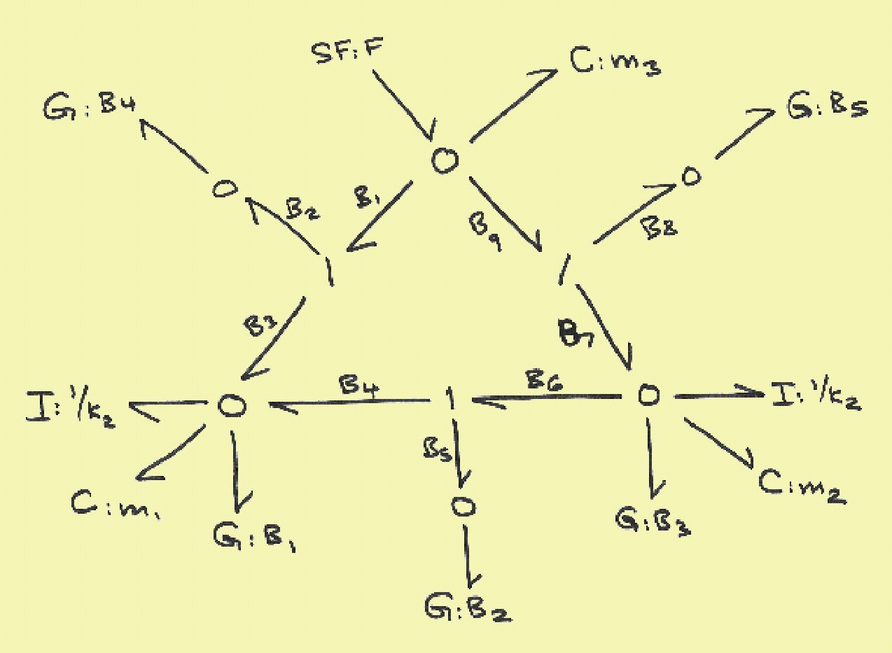
   4. Extract a complete set of causal equations representing this bond graph.

      We can read out from the bond graph the following equations directly:

      

    

4. We consider the crane crab example of Chapter 4 of the book:

   

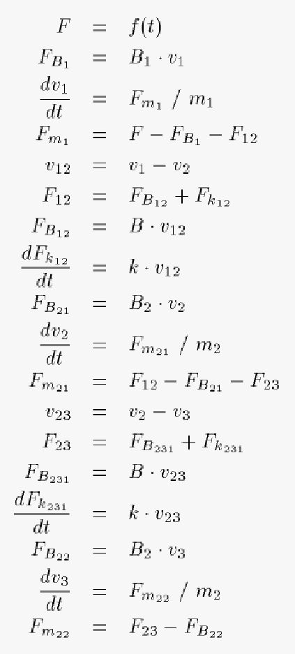
   The equations describing this system were:

   

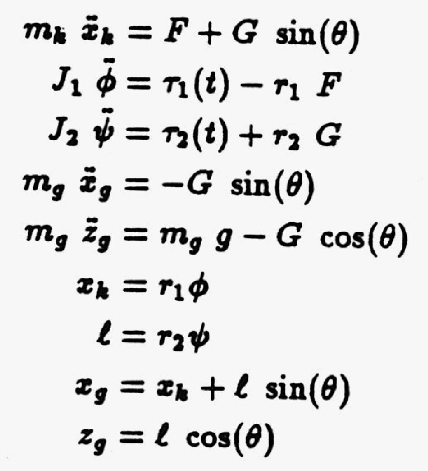
   We wish to construct a bond graph for this system.

   The four constraint equations need to be differentiated once:

   

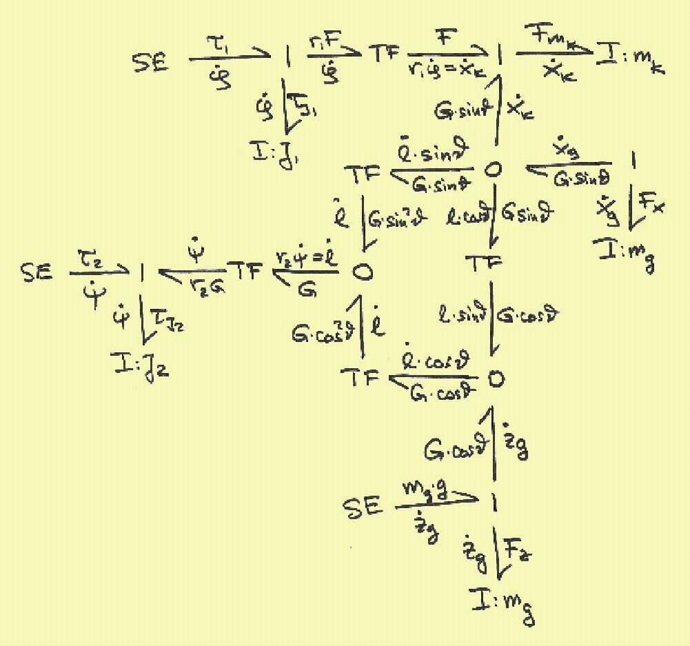
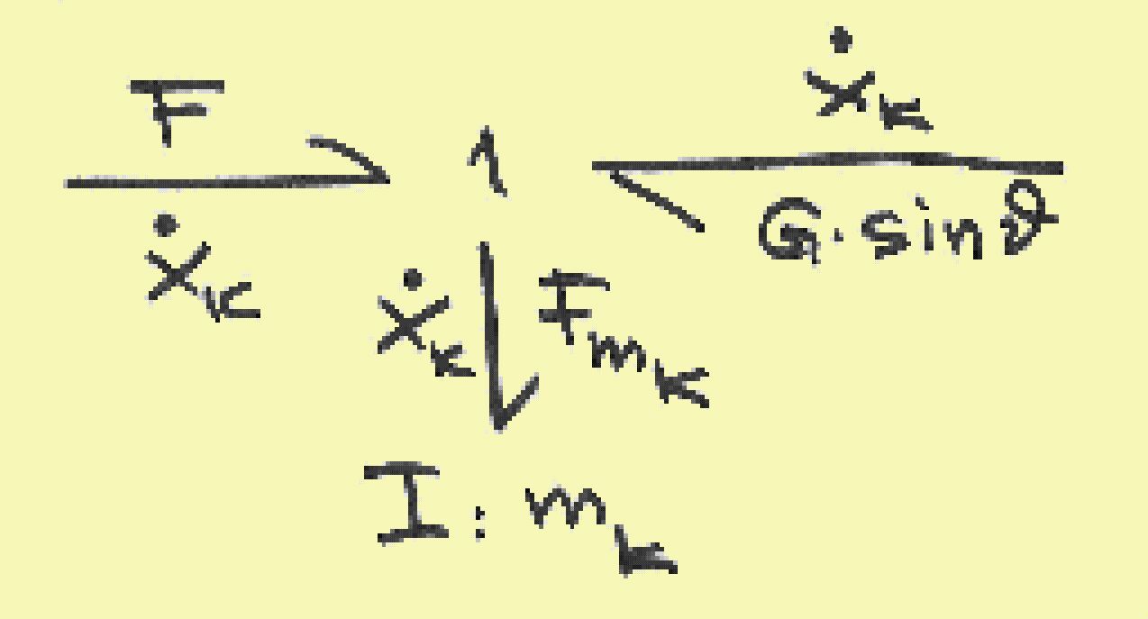
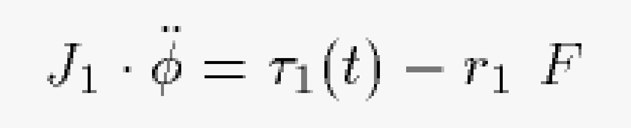
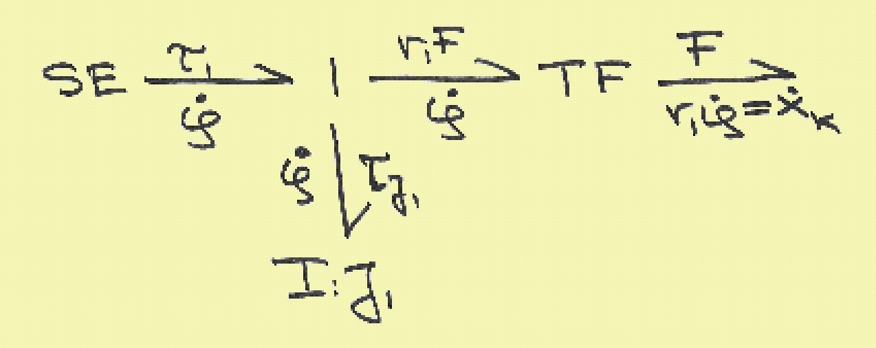
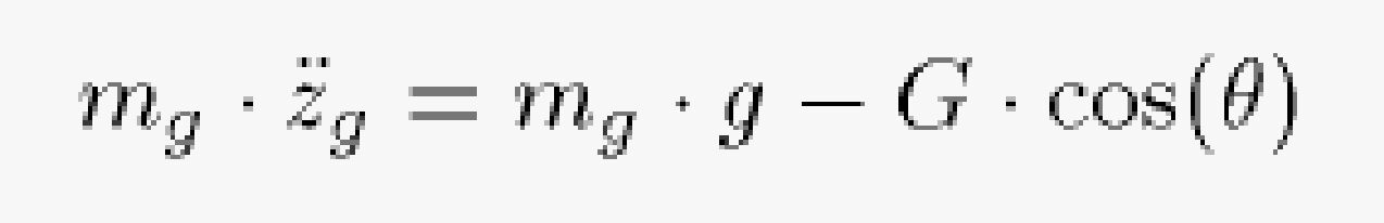
   We start by formulating bond graphs for each of the five Newton laws. Let us start with the first one:

   

   This equation describes a sum of forces, i.e., represents a 1-junction. Luckily, we know the flows associated with this 1-junction: the velocity of the body described by newton's law.

   

   Similarly for the second equation:

   

   

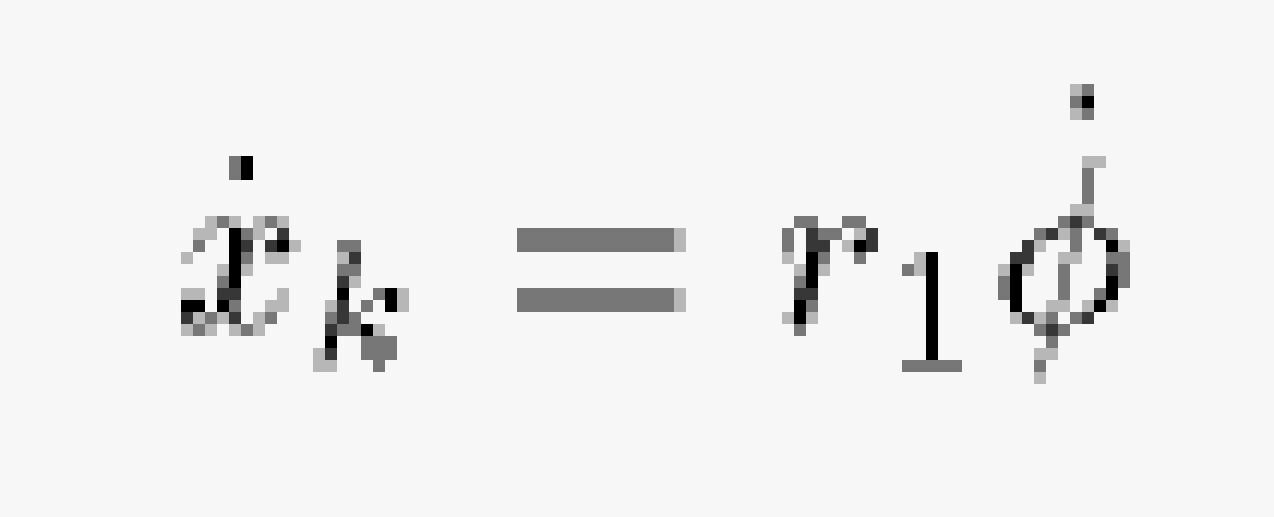
   The transformer represents one of the differentiated constraint equations:

   

   Evidently, the first bond graph can be placed snuggly to the right of the second.

   For the third equation, we find:

   

   

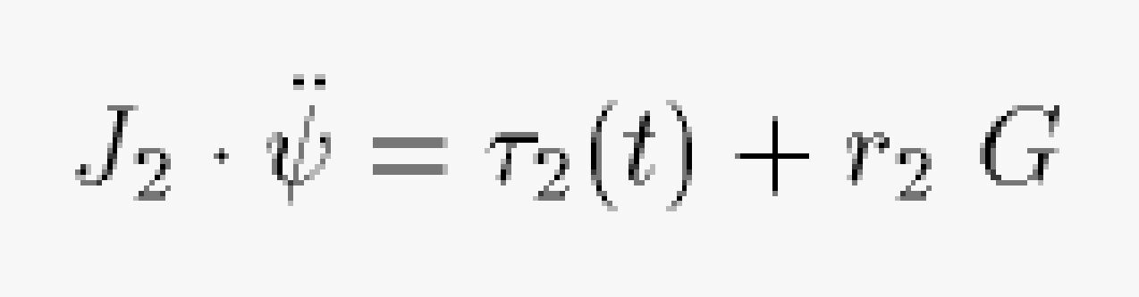
   The transformer represents another of the differentiated constraint equations:

   

   The fourth equation is:

   

   

   The fifth equation takes the form:

   

   

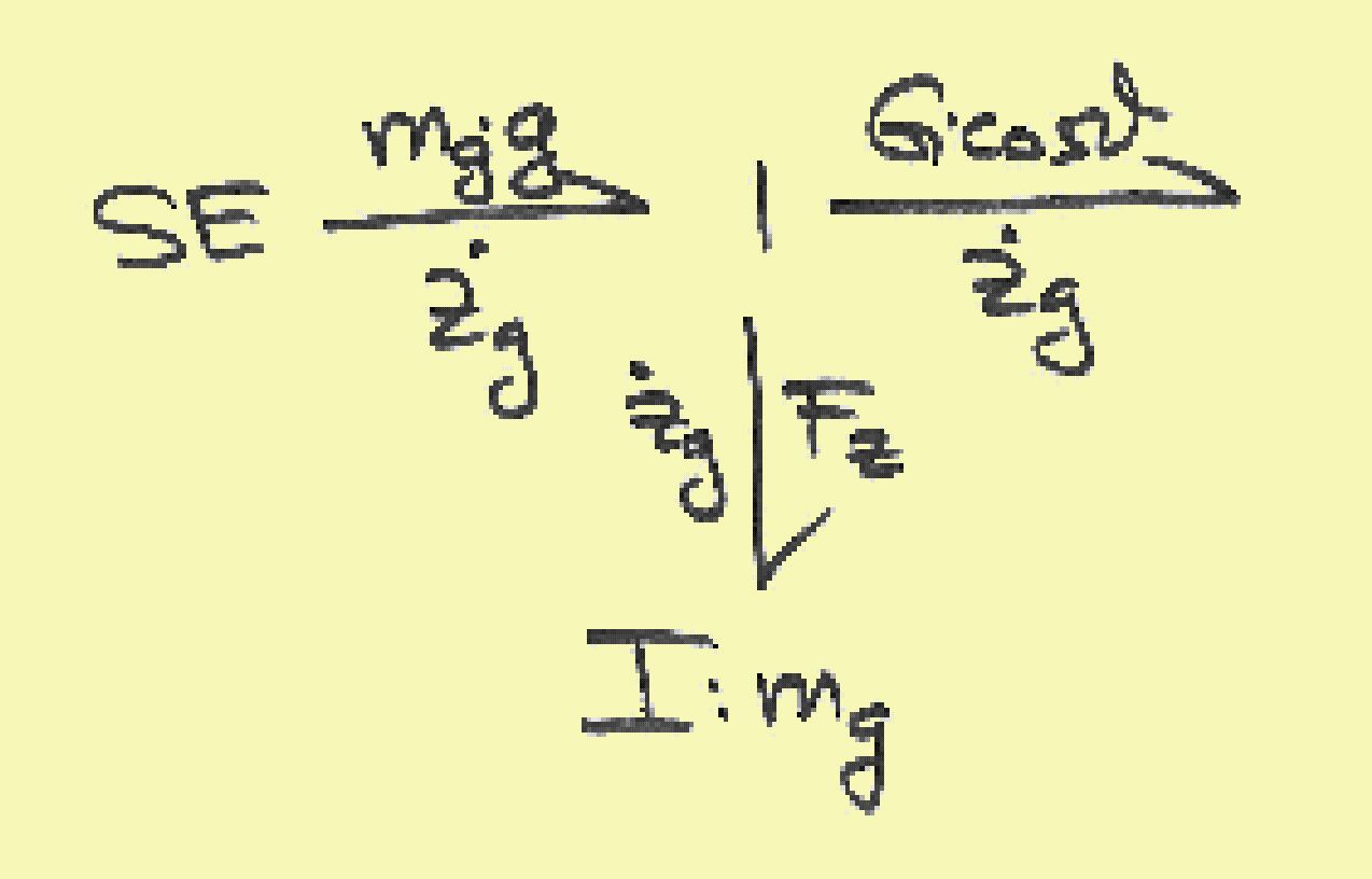
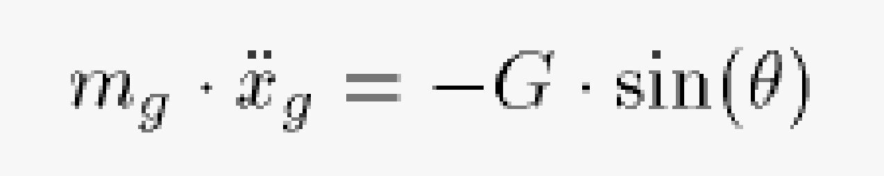
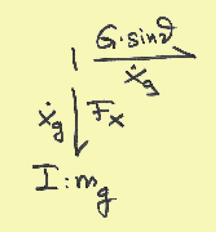
   The two remaining constraint equations represent sums of velocities, i.e., 0-junctions. Unfortunately, we don't know what the corresponding efforts should be. Let us start with the first of these differentiated constraint equations:

   

   Let's go shopping in the bond graphs for unresolved bonds. We find the velocity v_g associated with the effort G*sin(q). We also find the velocity v_k associated with the same effort. Hence it is a safe bet that this is the effort that needs to be associated with the bonds surrounding this 0-junction:

   

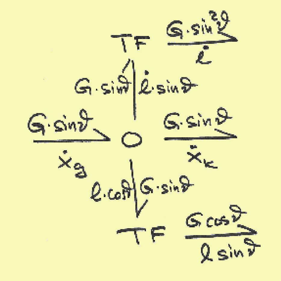
   The two transformers were added later, because it turns out that this is what we needed to connect some of the remaining unresolved bonds. The other remaining differentiated constraint equation is:

   

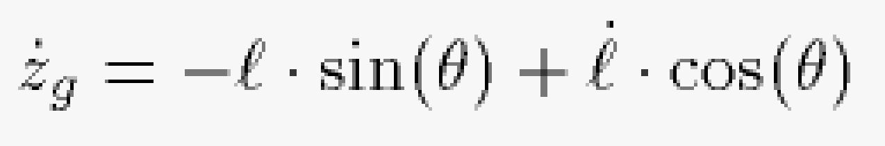
   Again, we don't know the associated effort yet. Shopping in the bond graphs, we find an unresolved bond assocated with the velocity in z-direction is G*cos(q). Hence we can draw the bond graph:

   

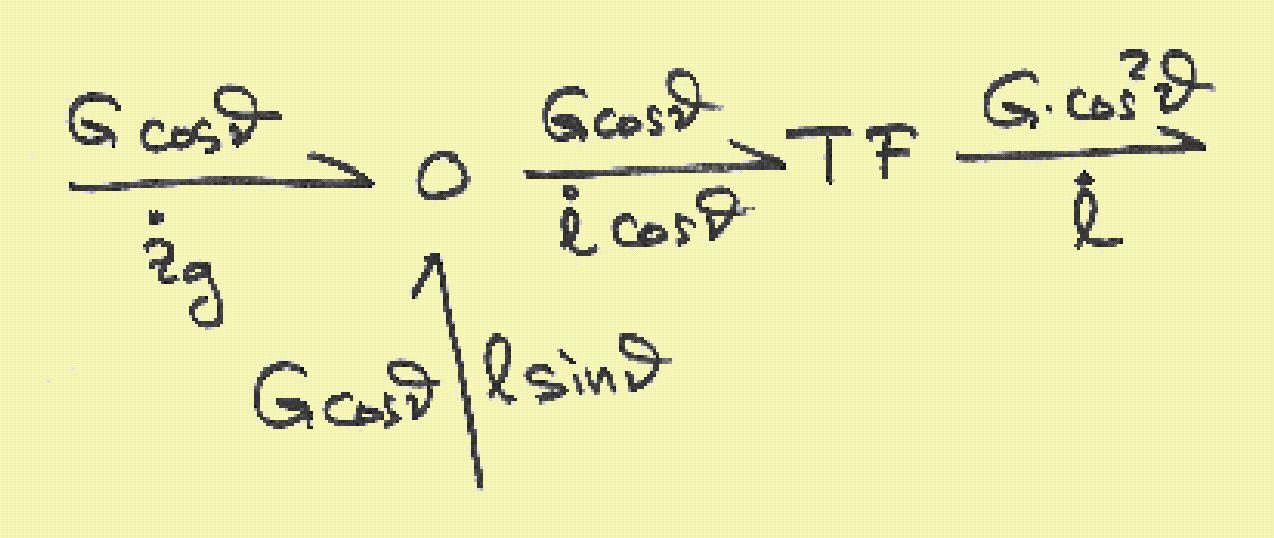
   Again, the transformer is used later.

   We remember the trigonometric relationship:

   
             sin2x + cos2x = 1
         

   We can use it in another 0-junction:

   

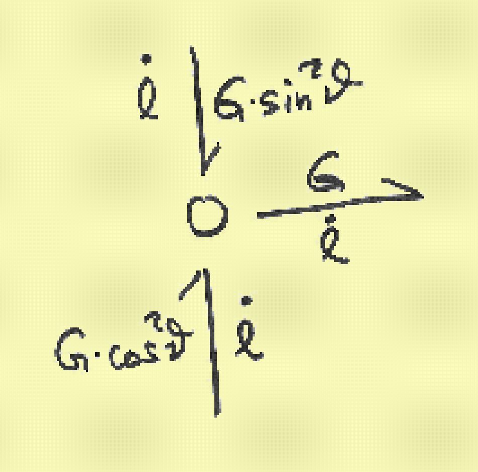
   Now, we have all the pieces of the puzzle. We can plug everything together, and obtain the bond graph: