AUDIO (WAV) FILES
A. Various WAV files used in class
Sampling rate: 11025Hz, 8-bits/sample.
"Your
work is ingenious..."
Sampling rate: 11025Hz, 8-bits/sample.
"How
soon can you land?..."
Sampling rate: 16000Hz, 16-bits/sample.
"Guitar
note: Standard A above middle C (440Hz pitch) played at 5th fret, high E string"
Sampling rate: 16000Hz, 16-bits/sample.
"Short
blues phrase"
Sampling rate: 16000Hz, 16-bits/sample.
"1999"
Sampling rate: 16000Hz, 16-bits/sample.
"Sur
Vesdre"
Sampling rate: 44.1kHz, 16-bits/sample.
"Purify"
Sampling rate: 44.1kHz, 16-bits/sample.
"Lick"
DATA FOR MATLAB PROJECT II
Sampling rate: 44.1kHz, 16-bits/sample.
"allplusaaa"
"aaanote"
B. Digital audio effects
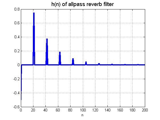
The following allpass reverb filter (Lesson
24) was implemented in Matlab as follows:
[x,Fs,bits]=wavread('duet_dry'); duet_dry
b=[-0.02 zeros(1,3000) 1]; a=[1 zeros(1,3000) -0.02];
y=filter(b,a,x);
sound(y,Fs)
wavwrite(y,Fs,bits,'duet_rvb'); duet_rvb
Filter h(n) plot
These were produced by playing a guitar
through a Korg G3 guitar effects pedal.
Chorus1
Chorus2
Flange
Flange22
Reverb
Reverb2
Here is another example of the chorusing effect: Snowmen
Chorus
These reverb effects were produced using
a Digitech RP350 guitar effects pedal. Use them as a reference for Matlab Project
I.
No
Reverb
Room
Reverb
Concert
Hall Reverb
This is the
original speech from the movie Amadeus. Sampling rate: 11025Hz, 8-bits/sample.
Hence data rate = 88kbits/s.
Original
8-bit PCM data: "Your work is ingenious..."
Next, each data frame is synthesized using
an IIR filter whose coefficients were computed from the speech data. The filter
is excited using an impulse train with constant spacing between impulses, simulating
speech at a constant pitch. (Robotic sounding.)
Result
of linear predictive coding with impulses giving completely voiced
speech at a constant pitch period
Here, white noise is used as the excitation.
The whisper-like synthetic speech is perfectly intelligible.
Result
of linear predictive coding with white noise giving completely unvoiced
speech
Here we have LPC as it was intended, with mixed excitation
and pitch resulting from software that makes voicing decisions and detects the
pitch period of voiced frames. Compressed data rate ~4kbits/s.
Result
of linear predictive coding with voicing decisions and variable pitch
Here the LPC code that was used to synthesize the Amadeus
speech is applied to speech from Sean Connery in Hunt for Red October.
The quality is poor, even though both speech signals use the same sampling rate
of 11025Hz. The pitch of the two actors' voices is quite different, and this
likely affects the results. The challenge is to write LPC code that is not so
data dependent.
Here we have LPC as it was intended, with mixed excitation
and pitch resulting from software that makes voicing decisions and detects the
pitch period of voiced frames. Compressed data rate ~4kbits/s.
Second
input signal
Result
of linear predictive coding with voicing decisions and variable pitch, applied
to the second input signal
D. The sound of aliasing
This is the
original speech from the movie Amadeus. Sampling rate: 11025Hz, 8-bits/sample.
Hence data rate = 88kbits/s.
Original
8-bit PCM data: "Your work is ingenious..."
After downsampling by a factor of 2. (Shown
in Lesson 19 as a box with a downward arrow followed by the number 2.) After
discarding every other sample, the new sampling rate is 11025/2 = 5512.5Hz.
Notice how aliasing distorts the high frequencies, notably the "s"
sounds. The MATLAB code was:
[x,fs,bits]=wavread('cutafew');
y=upfirdn(x,[1],1,2);
wavwrite(y,fs/2,bits,'downsample_by_2');
Aliased
after X2 downsampling
After downsampling by a factor of 4. (Shown in Lesson
19 as a box with a downward arrow followed by the number 4.) After discarding
3 out of every 4 samples, the new sampling rate is 11025/4 = 2756.25Hz. The
aliasing distortion is more pronounced.
[x,fs,bits]=wavread('cutafew');
y=upfirdn(x,[1],1,4);
wavwrite(y,fs/4,bits,'downsample_by_4');
Aliased
after X4 downsampling
After downsampling by a factor of 8. (Shown in Lesson
19 as a box with a downward arrow followed by the number 8.) After discarding
7 out of every 8 samples, the new sampling rate is 11025/8 = 1378.125Hz. The
intelligibility of the entire phrase is now severely compromised.
[x,fs,bits]=wavread('cutafew');
y=upfirdn(x,[1],1,8);
wavwrite(y,fs/8,bits,'downsample_by_8');
Aliased
after X8 downsampling
Finally, it's fun to listen to the speech after downsampling,
but played back at the original rate of 11025Hz. You will hear three consecutive
renditions (with short pauses separating them) of data downsampled by 2, 4 and
8. Only the first is intelligible in a chipmunk-like way. Perhaps humming birds
can understand the last two!
The
Chipmunks do Mozart
This example illustrates Lesson 3, page 4. Using a fixed
sampling rate of 6kHz, the input CT sinusoid is swept in frequency from 0-6kHz
(a "chirp" signal) during a 10s time window. No aliasing occurs from
0-3kHz. From 3-6kHz, we hear an alias frequency that is the reflection (or folding)
of the input frequency about the "wall" that occurs at 3kHz (the folding
frequency). As seen in the notes, this alias frequency swoops down from 3kHz
down to 0. The code that generated these WAV examples is:
function aliasplay(Fs,tmax,Fmax)
% function aliasplay(Fs,tmax,Fmax)
% Listen to aliasing as sinusoid freq is swept as a ramp function
% Fs - sampling freq
% tmax- length of sweep
% Fmax - height of ramp
T=1/Fs;t=0:T:tmax;freqin=(Fmax/tmax)*t;
x=chirp(t,0,tmax,Fmax); plot(t,freqin);xlabel('secs');ylabel('Hz');title('Input
freq vs time');grid
wavwrite(x,Fs,16,'alias');
sound(x,Fs)
0-6kHz
chirp signal sampled and played back at a sampling rate of 6kHz
This is the same as the previous example except that
the input frequency is swept from 0-12kHz in 10s, so we hear the output frequency
go up and down twice.
0-12kHz
chirp signal sampled and played back at a sampling rate of 6kHz
E. The sound of quantization noise (few bits/sample)
This is the
original speech from the movie Amadeus. Sampling rate: 11025Hz, 8-bits/sample.
Hence data rate = 88kbits/s.
Original
8-bit PCM data: "Your work is ingenious..."
MATLAB writes WAV files with a minimum of
8-bits/sample, so I concocted the following code to quantize my data into 4
bits/sample (that's only 16 quantization levels).
[x,fs,bits]=wavread('cutafew');
y=double(uencode(x,4));
y=y/max(y);
y=2*(y-0.5);
d=x-y; % Quantization noise
plot(d)
sound(y,fs) % Listen to 4-bit speech
sound(d,fs) % Listen to quantization noise
wavwrite(y,fs,8,'4bit_speech');
wavwrite(d,fs,8,'4bit_quantization_noise');
The quantization noise is by no means totally random. Parts sound like wideband
(~white) noise in the background of the signal. Between words, the noise has
a structured (buzzing) quality as the quantizer cycles between levels adjacent
to 0.
Speech
quantized to 4 bits/sample
Listen to just the quantization noise. Clearly,
using a white noise model for quantization noise is a fairly crude approximation.
4-bit
quantization noise
F. Sounds of filtered white noise
All filters were created using the MATLAB
function FIR1. Each filter contained 1001 coefficients, yielding a sharp cutoff
at the band edge(s).
This is 0-4kHz white (flat power spectrum) noise,
played at 8kHz sample rate, and 8-bits/sample. (No filtering.)
White
noise
White noise filtered using a 0-2KHz bandwidth
lowpass filter. Notice the perceptible 2kHz whistle. Sharp-cutoff audio filters
are known to generate such "ringing" at the band-edge frequencies.
0-2kHz
lowpass noise
White noise filtered using a 0-400Hz bandwidth
lowpass filter. Good wind-sound synthesizer?
0-400Hz
lowpass noise
White noise filtered using a 400Hz bandwidth
bandpass filter centered on 2kHz (i.e. 1800-2200Hz). Notice the rather complex
whistling with potential components at 2kHz as well as the band edge frequencies.As
the noise bandwidth increases, this tonality becomes less obvious and the crackle/hiss
quality grows.
1800-2200Hz
narrowband noise
White noise filtered using a 2-4KHz highpass
filter.
2-4kHz
highpass noise
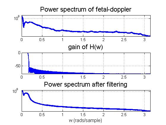
G. Filtering a fetal heartbeat signal
This original fetal doppler signal contains
significant noise. (Fs=22050Hz, Nbits=16).
Fetal
doppler
A length-1001 FIR filter was designed after examining the power spectrum of
the original signal, using the code: P=psd(x); semilogy(P). Rather than me tell
you the type and bandwidth of the filter used, download the original signal
and try designing your own filter. (Hint: I used the MATLAB commands FIR1 and
CONV.)
Filtered
doppler Plot
of spectra and filter used
H. Measuring vocal pitch
Excerpt from Mariah Carey singing the national
anthem at the 2002 Super Bowl. (Fs=44100Hz, Nbits=16.)
Land
of the free
Very short excerpt from her high note "...land of the FREE." Vocal
pitch measured at 1838Hz, corresponding to a note of ~A6# (1865Hz). The pitch
measurement technique will be discussed in Lesson 9. See Autocorrelation
plot .
FREEEEEE
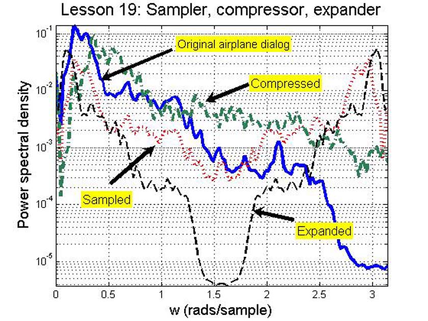
I. Sampler, compressor, expander (Lesson 19)
This is the original signal. Sampling rate:
11025Hz, 8-bits/sample.
"How
soon can you land?..."
After "sampling" i.e. setting all odd numbered
samples to zero. Playback rate: 11025Hz, 8-bits/sample.
Sampled
After "compression" i.e. discarding every other
sample with no zero-insertion. Playback rate: 5512.5Hz, 8-bits/sample.
Compressed
After "expansion" i.e. inserting a zero between
all samples. Playback rate: 22050Hz, 8-bits/sample.
Expanded
Power
spectra computed from the above files (Compare
the shape of these with the plots in the notes for Lesson 19.)
J. Simple sample-differencing filter & variable delay echo filter (Lesson 8)
See Lesson 8, page 5
Original audio signal. Sampling rate: 16000Hz,
16-bits/sample.
"1999"
LDE of adjacent-sample-differencing FIR
filter: y(n) = 0.5x(n) - 0.5x(n-1). Listen to how the low frequencies have been
reduced, and the high frequencies emphasized.
"Sample-difference
filter output"
LDE of long-echo-FIR filter: y(n) = x(n)
+ 0.5x(n-DELAY). The DELAY (in samples) is equivalent to 250ms or 500ms. The
250ms echo could perhaps be used as a cheap digital audio effect? The 500ms
echo is too long for musical applications.
"250ms
Echo Filter output"
"500ms
Echo Filter output"
K. Aliasing of sinusoidal chirp signal (Lesson 39, p. 3)
Sampling rate: 8000Hz, 16-bits/sample. The
frequency heard goes up, down, up and part-way down, as predicted by the graph
in Lesson 39, p. 3. The Matlab code is:
Fs=8e3; T=1/Fs; t= 0:T:10;
x=chirp(t,0,10,14e3);
sound(x,Fs)
"Chirping"
Last Modified: April 24, 2009